This file presents a discussion of the semi-log regression model. For an empirical example and additional discussion, please look at An empirical semi-log model of wages

The Semi-Logarithmic Function

The semi-logarithmic functional form is commonly used in econometrics because its coefficients represent useful concepts that are easily interpreted. To illustrate some basic properties of this specification consider the following model:

where P is the market price of a house, S is the size of the house in square feet, D is a dummy variable that takes the value of 1 if the house has a garage (zero otherwise) and T is a time trend variable that has values 1, 2 , 3,...., 36. T indicates in which of 36 consecutive months the house sold. The dependent variable in equation [1] is the natural logarithm of price. To examine the how the right hand side variables affect the Price of a house we need to take the exponential of both sides of [1] since the exponential function gives the anti-log of the natural logarithm:

Equation [3] is derived from [2] by using the fact that exp(a + b) = exp(a)exp(b).

Interpreting Coefficients: Continuous Variables

In this section it will be shown that the coefficient on the continuous variable S, (size) represents the effect of a change in S on price. More specifically, b₁ is the percentage change in P (price) that follows from a unit change in size. For example if b₁ = 0.02, a one square foot increase in size will raise price by 2%. This price response is identical for houses of all sizes, identical for all dates T and is the same for houses that have a garage (D = 1) and for houses that have no garage (D = 0).

One way to show this result is to differentiate P with respect to size, S. Recall that if

The last line shows that b is the percentage change in y per unit change in x. When this idea is applied to equation [2] we get

An alternative way to derive this results is to consider the effect of a small change in size, S on price. Label the resulting change in price as P. From equation [3] we have: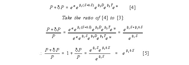

The left hand side of [5] represents one plus the percentage change in P since the denominator is the initial value of P and the numerator is the initial value plus the change in P. When S is set to 1, equation [5] implies that the percentage change in P is exp(b₁) - 1. A scientific calculator confirms that for small values of x, exp(x) - 1 @= x (Here, @= means "approximately = to"). For example, if x = 0.01, exp(x) @= 1.01005 and if x = .03, exp(x) @= 1.0305. These examples confirm that if the coefficient b₁ is small, it represents the percentage change in P that results from a unit change in S.

Interpreting Coefficients: Dummy Variables

In this section we show that b₂, the value of a garage, is the coefficient on D in the sense that the percentage difference in the prices of houses that have garages compared to those that do not is b₂. This percentage difference is the same for houses of all sizes and it is

independent of time. For houses that have a garage, D = 1 and for those that do not, D = 0. We can use equation [3] to calculate the ratio of the prices of these two types of houses.

Since the ratio of prices is approximately (1 + b₂) the percentage increase in price due to the presence of a garage is approximately b₂. For example if b₂ = 0.06 then a garage raises the price of a house by approximately 6%.

Interpreting Coefficients: The Time Trend

The theory that has been presented above applies directly to the time trend coefficient which represents the percentage increase in price that follows from a unit increase in T. When the frequency of time is measured in months, as in the current example, a unit increase in T means that one month has passed so the coefficient on T represents the monthly percentage increase in prices. This percentage increase is the same for every month within the sample and is the same for houses of all sizes with or without garages. This conclusion follows from the fact that the derivative

is simply equal to b₃ and is therefore independent of T, S and D.